| All in one page | Postscript version | PDF version |
| Previous chapter: 2. QKG versus courier | Abstract and TOC | Next chapter: 4. Entropy |
| All in one page | Postscript version | PDF version |
| Previous chapter: 2. QKG versus courier | Abstract and TOC | Next chapter: 4. Entropy |
For the current purposes it is sufficient to think of a
discrete random variable ![]() as variable with a fixed but unknown integer
value larger than or equal to zero. The random variables we will
encounter later will be mostly secret keys, messages, and message
tags. Our knowledge about the random variable is completely
determined by a vector of positive probabilities
as variable with a fixed but unknown integer
value larger than or equal to zero. The random variables we will
encounter later will be mostly secret keys, messages, and message
tags. Our knowledge about the random variable is completely
determined by a vector of positive probabilities
![]() , each describing how
confident we are that the variable's value is the specific
integer
, each describing how
confident we are that the variable's value is the specific
integer ![]() , adding
up to 1. It is often better to talk about uncertainty, or
entropy, instead of knowledge. No uncertainty means full
knowledge, i.e., 100% probability for one value and 0% for the
rest.
, adding
up to 1. It is often better to talk about uncertainty, or
entropy, instead of knowledge. No uncertainty means full
knowledge, i.e., 100% probability for one value and 0% for the
rest.
An important special case is the random variables for which all non-zero probabilities are equal. These random variables are called uniform random variables. If Alice throws a normal, but perfect, six-sided die and keeps the result secret, the result is to Bob a uniform random variable with six possible values. If Bob had managed to replace Alice's die with one that is not perfect, the variable would not have been completely uniform. In any case, Alice knows the value so to her it is a random variable with zero uncertainty or entropy.
The range of ![]() is
the set of values
is
the set of values ![]() can
have, even those with zero probability, and is denoted
can
have, even those with zero probability, and is denoted
![]() . Even though
infinite ranges are possible, we will limit ourselves to random
variables with finite ranges. Without loss of generality we will
only consider ranges consisting of integers
. Even though
infinite ranges are possible, we will limit ourselves to random
variables with finite ranges. Without loss of generality we will
only consider ranges consisting of integers ![]() .
.
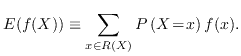
The expectation value is denoted ![]() and can be defined as
and can be defined as
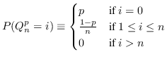
Throughout the rest of this thesis the class of random
variables ![]() defined by (3.2) will serve as an
illustrative example. The same definition in Python code is
available as function Q in entropies.py line 54 .
defined by (3.2) will serve as an
illustrative example. The same definition in Python code is
available as function Q in entropies.py line 54 .
![]() is a uniform
random variable with
is a uniform
random variable with ![]() possible values. If
possible values. If ![]() is large
is large ![]() has one very probable and
has one very probable and
![]() equally
improbable values. Such random variables are rather extreme and
will therefore nicely illustrate some somewhat unintuitive
situations later.
equally
improbable values. Such random variables are rather extreme and
will therefore nicely illustrate some somewhat unintuitive
situations later.
Two random variables ![]() and
and ![]() can be related in ways that are unrelated to
their internal probability vectors. To completely specify both
their respective probability vectors and their relations it is
sufficient (and necessary) to (be able to) specify the
probability vector of a larger random variable, the concatenation of the two variables, written as
can be related in ways that are unrelated to
their internal probability vectors. To completely specify both
their respective probability vectors and their relations it is
sufficient (and necessary) to (be able to) specify the
probability vector of a larger random variable, the concatenation of the two variables, written as
![]() , with
probabilities
, with
probabilities
![]() and
and ![]() . Observe that neither
. Observe that neither ![]() nor
nor ![]() are products. When the random
variables are related in this way the probabilities in their
respective smaller probability vectors are called marginal probabilities.
are products. When the random
variables are related in this way the probabilities in their
respective smaller probability vectors are called marginal probabilities.
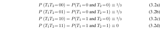
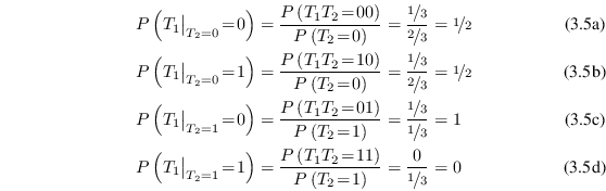
As an example, consider the dependent random variables defined by
 |
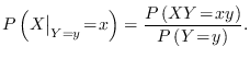
Given two random variables ![]() and
and ![]() , when learning that the value of
, when learning that the value of
![]() is
is ![]() the probability vector of
the probability vector of
![]() can change. If
they are dependent
can change. If
they are dependent ![]() contains information about
contains information about ![]() and receiving information changes the
probabilities. The new random variable can be denoted
and receiving information changes the
probabilities. The new random variable can be denoted
![]() and
its probability vector is
and
its probability vector is
This relation is called Bayes' theorem and is a fundamental part of probability theory, but the notation is unorthodox.
Normally
![]() is written as
is written as
![]() and is read as
the probability that
and is read as
the probability that ![]() equals
equals ![]() given that
given that ![]() equals
equals ![]() . Similar notations are
used for other things, most notably for conditional entropy. We
will use the unconventional notation exclusively, both to note
explicitly that we are working on a new random variable and to
bring the implicit hidden expectation value in conditional
entropy written the conventional way out into the light. See
Chapter 4.4.1 for more
details.
. Similar notations are
used for other things, most notably for conditional entropy. We
will use the unconventional notation exclusively, both to note
explicitly that we are working on a new random variable and to
bring the implicit hidden expectation value in conditional
entropy written the conventional way out into the light. See
Chapter 4.4.1 for more
details.
Using Bayes' theorem on the previously defined ![]() and
and ![]() yields
yields
 |
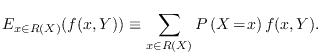
With more than one random variable it can be necessary to specify the expectation value over just one of them. A natural definition is
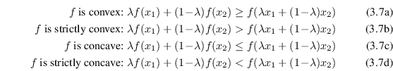
There are lots of standard inequalities that are very useful in connection with random variables. We will only need one of them, Jensen's inequality.
Jensen's inequality is applicable to convex and concave
functions. A function is called convex if it is continuous and
the whole line between every two points in its graph lies on or
above the graph. If the whole line lies above the graph it is
also called strictly convex. A function ![]() is concave3.1 or
strictly concave if
is concave3.1 or
strictly concave if ![]() is convex or strictly convex. In other words,
for all
is convex or strictly convex. In other words,
for all
![]() ,
,
![]() , and
, and
![]() holds:
holds:
 |
Jensen's inequality states that if
![]() is a convex or
concave function, then for any random variable
is a convex or
concave function, then for any random variable ![]() :
:
 |
For a random variable with only two possible values, Jensen's inequality just restates the definition of convexity. Generalizing to arbitrary number of values by induction is pretty straightforward and is explained in many other places.
If ![]() is
convex and has an inverse, an alternative way to express Jensen's
inequality is
is
convex and has an inverse, an alternative way to express Jensen's
inequality is
![]() .
.
| All in one page | Postscript version | PDF version |
| Previous chapter: 2. QKG versus courier | Abstract and TOC | Next chapter: 4. Entropy |