| All in one page | Postscript version | PDF version |
| Previous chapter: 3. Discrete random variables | Abstract and TOC | Next chapter: 5. Unconditionally secure authentication |
| All in one page | Postscript version | PDF version |
| Previous chapter: 3. Discrete random variables | Abstract and TOC | Next chapter: 5. Unconditionally secure authentication |
Entropy is an important concept in many fields, and one field where it is extensively used is QKG. This chapter gives a general overview of entropy and presents a generalization of the chain rule of entropy as needed in future chapters. Alternate explanations to most of the contents can be found in many other places, along with lots of other useful bounds and relations. The introductory chapters of [6] are highly recommended.
The function
![]() where
where ![]() is a
probability occurs frequently in connection with entropies.
is a
probability occurs frequently in connection with entropies.
![]() is
normally undefined but since
is
normally undefined but since
![]() is well-defined we extend
the function to zero by continuity.
is well-defined we extend
the function to zero by continuity.
Another convention we will follow is to let
![]() mean
the logarithm base 2. We can choose any base, but using base 2
consequently means that everything will be expressed in bits, and
people tend to be familiar with bits.
mean
the logarithm base 2. We can choose any base, but using base 2
consequently means that everything will be expressed in bits, and
people tend to be familiar with bits.
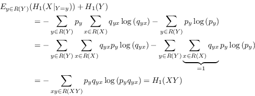
Entropy is a measure of uncertainty regarding a discrete random variable. For many purposes, the Shannon entropy is the only measure needed. Shannon entropy is defined by
The Shannon entropy is a fundamental measure in information theory. It was introduced by Claude E. Shannon, now considered the father of information theory, in [7]. Much can be said about its properties, its uniqueness, and its relation with the thermodynamical entropy in physics, but we will only scratch a little bit on the surface here. One way of understanding it better is to rewrite the definition as
Now it is clear that the Shannon entropy is the expectation
value of ![]() where
where ![]() is the
probability assigned to the measured value of the random
variable.
is the
probability assigned to the measured value of the random
variable. ![]() can be interpreted as the needed length, in bits, of a message
communicating a measurement that had probability
can be interpreted as the needed length, in bits, of a message
communicating a measurement that had probability ![]() , which makes the Shannon entropy
a measure of the expected message length needed to communicate
the measured value of a random variable.
, which makes the Shannon entropy
a measure of the expected message length needed to communicate
the measured value of a random variable.
The Shannon entropy of a uniform random variable with
![]() possible values
is
possible values
is
| (4.3) |
Without qualifiers, the word entropy and a non-subscripted
![]() normally refers
only to Shannon entropy. However, when dealing with QKG, as well
as most other parts of cryptography, this measure is not
sufficient. The goal of QKG is to produce a key that is known to
both Alice and Bob but to Eve is a random variable with high
uncertainty.
normally refers
only to Shannon entropy. However, when dealing with QKG, as well
as most other parts of cryptography, this measure is not
sufficient. The goal of QKG is to produce a key that is known to
both Alice and Bob but to Eve is a random variable with high
uncertainty. ![]() is a measure of the uncertainty of a
value assigned probability
is a measure of the uncertainty of a
value assigned probability ![]() and is therefore a measure of the security of
that particular value of the key. Shannon entropy measures the
expectation value of that security. The dangers of focusing on
Shannon entropy alone is highlighted by this theorem:
and is therefore a measure of the security of
that particular value of the key. Shannon entropy measures the
expectation value of that security. The dangers of focusing on
Shannon entropy alone is highlighted by this theorem:
 |
(4.4) |
which completes the proof. ![]()
Good security average is not good enough, and Shannon entropy alone is obviously not a sufficient measure of the quality of a key.
Another measure more closely related to the difficulty of
guessing the value of a random variable was introduced by Massey
in [8]. He did
not name it but in [6]
it is called guessing entropy. Note,
however, that while most other entropies have the unit
bits the guessing entropy is measured
in units of number of guesses.
Without loss of generality we can assume that the values of
![]() are sorted with
decreasing probability, in which case the guessing entropy of
are sorted with
decreasing probability, in which case the guessing entropy of
![]() is defined as
is defined as
 |
(4.6) |
Again we see that good security average is not good enough, and guessing entropy alone is not a sufficient measure of the quality of a key.
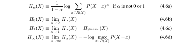
A useful generalization of Shannon entropy is the Rényi
entropy, which maps an entropy measure
![]() pronounced the Rényi entropy of order
pronounced the Rényi entropy of order
![]() to
every real number
to
every real number
![]() . Rényi entropy is,
just like Shannon entropy, measured in units of bits.
. Rényi entropy is,
just like Shannon entropy, measured in units of bits.
An important property of Rényi entropy is that for
![]() ,
,
![]() for all
for all
![]() , with equality if
and only if
, with equality if
and only if ![]() is a
uniform random variable. In other words,
is a
uniform random variable. In other words,
![]() is a
constant function of
is a
constant function of ![]() if
if ![]() is uniform and strictly decreasing if not. A
full proof is given in [6] and follows quite naturally
by writing
is uniform and strictly decreasing if not. A
full proof is given in [6] and follows quite naturally
by writing
![]() in
analogy with (4.2) as
in
analogy with (4.2) as
![]() and using Jensen's inequality.
and using Jensen's inequality.
Some of these measures have quite natural interpretations.
Rényi entropies with higher ![]() parameter depend more on the probabilities
of the more probable values and less on the more improbable ones.
parameter depend more on the probabilities
of the more probable values and less on the more improbable ones.
![]() is logarithm
of the number of values of
is logarithm
of the number of values of ![]() that have non-zero probabilities. Any two random
variables with different probability distributions but the same
number of values with non-zero probabilities will have the same
Rényi entropy of order 0.
that have non-zero probabilities. Any two random
variables with different probability distributions but the same
number of values with non-zero probabilities will have the same
Rényi entropy of order 0.
![]() is the
Shannon entropy, in which the actual probabilities are quite
important.
is the
Shannon entropy, in which the actual probabilities are quite
important.
![]() is often
called collision entropy, or just Rényi entropy, and is
the negative logarithm of the likelihood of two independent
random variables with the same probability distribution to have
the same value. More probable values are much more likely to
collide and are therefore more visible in the collision entropy
than in the Shannon entropy.
is often
called collision entropy, or just Rényi entropy, and is
the negative logarithm of the likelihood of two independent
random variables with the same probability distribution to have
the same value. More probable values are much more likely to
collide and are therefore more visible in the collision entropy
than in the Shannon entropy.
![]() is
called min-entropy and is a function of the highest probability
only.
is
called min-entropy and is a function of the highest probability
only.
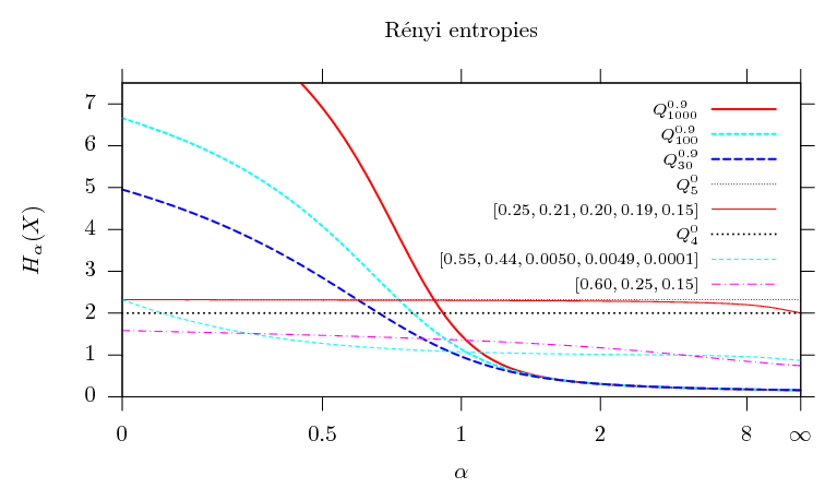
The shape of
![]() as a
function of
as a
function of ![]() for
eight different random variables
for
eight different random variables ![]() is shown in figure 4.1.
is shown in figure 4.1.
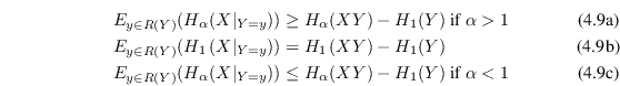
 |
(4.9) |
Rényi entropies of different order than 1 are not
expectation values so things are not quite as simple. In fact,
according to [6] there
is not even an agreement about a standard definition of
conditional Rényi entropy. However, the dominant
definition seems to be the same as (4.8) with both ![]() :s replaced by
:s replaced by ![]() . That definition will be
used here but the expectation value will always be explicitly
written out. We have seen that averaging security can be
dangerous, and it is nice to not hide away something potentially
dangerous in the notation.
. That definition will be
used here but the expectation value will always be explicitly
written out. We have seen that averaging security can be
dangerous, and it is nice to not hide away something potentially
dangerous in the notation.
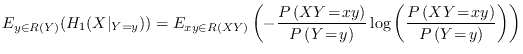
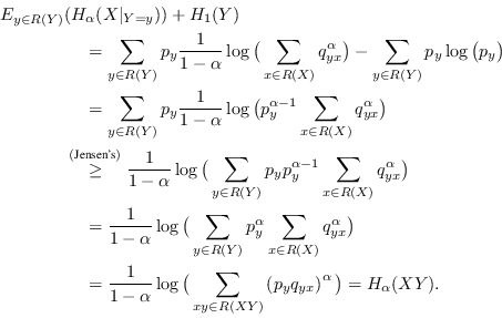
With conditional Shannon entropy comes the chain rule of Shannon entropy, equation (4.10b) below. One way to define conditional Rényi entropy is to choose it so the same relation still holds when the Shannon entropies are replaced with Rényi entropies. However, the relation does not hold for the expectation value based definition chosen above so it is clearly a different conditional entropy. Fortunately, that doesn't stop us from generalizing the chain rule in other ways to something that is useful with general Rényi entropies:
 |
(4.11) |
When ![]() we have instead:
we have instead:
 |
(4.12) |
When learning something new about a random variable, the
Shannon entropy of the variable will decrease or stay equal on
average. It is only true on average. Consider
![]() and a
and a ![]() that is
dependent on
that is
dependent on ![]() such that
such that ![]() if
if
![]() and
and
![]() if not.
Learning that
if not.
Learning that ![]() is
1 will increase the Shannon entropy of
is
1 will increase the Shannon entropy of ![]() from 0.15 to 6.64, but learning
that
from 0.15 to 6.64, but learning
that ![]() is 0
will decrease it to exactly 0. On average, the Shannon entropy
will decrease to 0.0664. On average, the Shannon entropy will
always decrease for all
is 0
will decrease it to exactly 0. On average, the Shannon entropy
will decrease to 0.0664. On average, the Shannon entropy will
always decrease for all ![]() and
and ![]() .
.
However, that is not true in general for other Rényi
entropies. For example, consider ![]() and
and ![]() defined in (3.3a).
defined in (3.3a).
![]() . If
. If
![]() turns out to be
1 the entropy of
turns out to be
1 the entropy of ![]() reduces to exactly 0, if not it becomes exactly 1. On average, it
will increase to
reduces to exactly 0, if not it becomes exactly 1. On average, it
will increase to
![]() .
.
Side information that increases entropy on average like this was first mentioned in [9] and is called spoiling knowledge.
The Concise Oxford English Dictionary [10] describes holism as
the theory that certain wholes are greater
than the sum of their parts. In a way, random variables
normally behave in a holistic way. To specify both ![]() and
and ![]() the whole probability vector for
the whole probability vector for
![]() is needed and
the size of
is needed and
the size of ![]() is
the size of
is
the size of ![]() multiplied by the size of
multiplied by the size of ![]() . This is one reason why Shannon chose to
primarily use a logarithmic scale in [7]. With a logarithmic scale
the multiplications can be treated as sums and the whole is just
the sum of the parts. Quoting Shannon: One
feels, for example, that two punched cards4.3 should
have twice the capacity of one for information storage, and two
identical channels twice the capacity of one for transmitting
information.
. This is one reason why Shannon chose to
primarily use a logarithmic scale in [7]. With a logarithmic scale
the multiplications can be treated as sums and the whole is just
the sum of the parts. Quoting Shannon: One
feels, for example, that two punched cards4.3 should
have twice the capacity of one for information storage, and two
identical channels twice the capacity of one for transmitting
information.
It should come as no surprise that an important property of Shannon entropy is that the total entropy of a system is never greater than the sum of the parts' entropies,
On the other hand, what might come as a surprise is that this
is not true in general for other Rényi entropies. There
exists ![]() and
and
![]() such
that
such
that
For example, consider ![]() and
and ![]() defined in (3.3a) again.
defined in (3.3a) again.
![]() but
but
![]() .
This is a case where the whole actually is greater than the sum
of the parts.
.
This is a case where the whole actually is greater than the sum
of the parts.
| All in one page | Postscript version | PDF version |
| Previous chapter: 3. Discrete random variables | Abstract and TOC | Next chapter: 5. Unconditionally secure authentication |