Authentication in quantum key growing
Jörgen Cederlöf
Quantum key growing, often called quantum cryptography or quantum key distribution, is a method using some properties of quantum mechanics to create a secret shared cryptography key even if an eavesdropper has access to unlimited computational power. A vital but often neglected part of the method is unconditionally secure message authentication. This thesis examines the security aspects of authentication in quantum key growing. Important concepts are formalized as Python program source code, a comparison between quantum key growing and a classical system using trusted couriers is included, and the chain rule of entropy is generalized to any Rényi entropy. Finally and most importantly, a security flaw is identified which makes the probability to eavesdrop on the system undetected approach unity as the system is in use for a long time, and a solution to this problem is provided.
- Keywords:
- Quantum key growing, Quantum key generation, QKG, Quantum key distribution, QKD, Quantum cryptography, Message authentication, Unconditional security, Rényi entropy.
1. Introduction
The history of cryptography has been an arms race between code makers and code breakers. Today the code makers are far ahead of the code breakers. Anyone with a computer and some knowledge can send and receive encrypted and signed messages, and nobody can decrypt them or produce false signatures within a reasonable time frame. At least not someone limited to using the computers and the publicly known algorithms of today, and limited to attacking the messages themselves rather than exploiting human errors and software bugs, compromising physical security or something similar.
We trust cryptography so much that it now is hard to imagine what a modern society without working cryptography would look like. Code breakers getting ahead in the race tomorrow would not mean the end of civilization, but we would have to rethink much of what we have come to depend on and there would be a lot of changes around us. Not entirely different from the computer problems that were feared to appear on the arrival of the new millennium, but this time making some small bug fixes in old computer code would not be enough, many systems would need to be redesigned completely, and some would simply not be possible anymore.
Nobody knows if the code breakers will be better than the code makers ever again, but some fear that it might happen within years or at least within decades. One threat is the advancement of quantum computers. A quantum computer can solve certain types of problems much faster than a conventional computer. Breaking cryptography is one of those problems, but making more secure codes is not. Quantum computers have been built, but fortunately for the code makers no quantum computer nearly large enough to be usable is expected to be possible to build in the immediate future. The fear that they will exist in the near future is however, even though it may not be well-founded, real. As is the fear that new mathematical tools will make code breaking much easier.
The primary cryptography tools used today are symmetrical encryption, symmetrical authentication, asymmetrical encryption, and digital signatures. In the first two, both the sender and the receiver have a copy of the same secret key. The other two are similar but the sender and the receiver have different related keys, of which only one needs to be secret. The difference between encryption and digital signatures/authentication is explained in Chapter 5. Methods of using one secret and one public key was a major breakthrough of cryptography, but all those risk being insecure if the code breakers gain enough computational or algorithmic power. Even worse, the future code breakers would also be able to decrypt old stored encrypted messages. Luckily, the first two cryptography tools have been mathematically proven to be unbreakable if they are done right, so no matter what breakthroughs the future brings us they will still be available. Unfortunately, to do them right requires the secret key to be very large and to be discarded after use. This is quite impractical and seldom done today, and it will be even harder if asymmetrical cryptography is no longer available.
Handling those large keys, especially without asymmetrical cryptography, is today considered too impractical for most people to even consider doing it. This is not very strange considering we have much simpler tools to accomplish the same thing. If those tools disappeared handling those large keys might still be more practical than living without cryptography. All that is needed is a good and fast random number generator, good storage media and trusted couriers. Since the keys are discarded after use, the couriers will need to bring new keys each time nothing is left of the old ones.
Quantum Key Growing is both a fascinating application of quantum mechanics and another way to solve the key distribution problem. By using some quantum mechanical properties of single photons two persons in two different places sharing a small secret key can make that key grow to a larger key, and anyone trying to intercept the key will be detected. Unlike most classical cryptography, QKG makes no assumptions about the computational capacity of the enemy. Instead, the security is based on the enemy being limited by the laws of quantum mechanics.
QKG is also often called Quantum Cryptography or Quantum Key Distribution. These expressions have given rise to the idea that the message to be encrypted or a chosen secret key is sent as quantum information, when in fact the secret key generated is pretty random. The expression Quantum Key Growing is less frequently used but also emphasizes that an initial shared secret key is needed for the process to work, something which is often forgotten in popular scientific explanations of QKG.
The typical key generation rate of QKG systems available today is, according to [1], very low, 1000 bits/s at best and often much lower. This bit rate is far too low to be usable in an unbreakable one-time pad system for most applications. Instead, QKG is often promoted as a way of enhancing the security of classical cryptography like AES through constantly replacing the encryption key with fresh ones from the QKG system. This will of course invalidate any claims of unconditional security, since the encryption will be breakable to an eavesdropper with large enough computing power or good enough algorithms, but it is often argued that this is good enough security.
However, providing good enough security is necessary but not sufficient. It must also be as cheap and good as other ways to achieve the same or better level of security. Chapter 2 compares QKG with the less interesting but old and well-tried method of simply sending the key with a courier.
There are many different ways to implement a QKG system. See [2] for a very good review. This chapter will give a brief description of the basics. A good and detailed description of an example QKG system can be found in [3]. Chapter 3 introduces discrete random variables, Chapter 4 discusses different definitions of the entropy contained in a discrete random variable and generalizes the chain rule of entropy. Unconditionally secure authentication with a completely secret authentication key is explained in Chapter 5, and in Chapter 6 the key is allowed to be only partly secret. A vulnerability is identified and solutions are presented. Finally, Chapter 7 describes how the results apply to QKG. Much of what is explained in these chapters is also given as Python source code in appendix A.
1.1 Setup
Whenever cryptography is involved, it is common practice to refer to the sender, receiver and eavesdropper as Alice, Bob and Eve, respectively. If the eavesdropper is allowed to modify messages as well she is sometimes called Mallory, but most of the time, and here, she will be called Eve.
To set up a QKG system Alice and Bob need one quantum channel between them where they can send and receive quantum bits, qubits, from Alice to Bob. The channel is typically an optical fibre carrying single photons with the qubit coded in the photon's polarization, but many other possibilities exist. In a perfect channel every qubit sent by Alice is received and correctly measured by Bob, to the extent permitted by quantum mechanics, and Bob receives no qubits which Alice has not sent. In practice, such channels don't exist, and they are not needed. The actual channel used can lose almost all qubits in transit, make Bob think he received qubits never sent by Alice and modify some of the qubits that do go from Alice to Bob. As long as the errors are within some limits QKG will still produce a key that is both shared and secret.
They will also need one classical information channel. The alternatives include but are not limited to the Internet, the same optical fibre used above, and a network cable parallel to the optical fibre. Note that many descriptions describe a system where messages on the classical channel can be eavesdropped but can never be modified by Eve. Such a system merely turns a quantum channel and an unmodifiable channel into a channel safe from eavesdropping. Such unmodifiable channels don't exist in the real world, and they are not needed. In reality, Eve must be assumed to have complete control over the classical channel as well as the quantum channel. Using message authentication Alice and Bob can detect Eve's modification attempts with a high probability. Message authentication is the topic of this thesis.
Alice and Bob will also need a shared secret key to begin with. It does not need to be very large at first, the sole purpose of the QKG system is to make this shared key grow by using and discarding small parts of it to produce larger keys. The initial key only needs to be large enough to enable the message authentication needed to create a larger key, which typically would mean being able to authenticate two messages, one from Alice to Bob and one in the other direction. Alice and Bob will also need random number generators, and of course computers.
1.2
Running the system
QKG was first proposed by Charles H. Bennett and Gilles Brassard in the paper [4] in 1984. The protocol they described is now known as BB84. They assumed that the quantum channel was perfect but they did describe how to do message authentication to prevent Eve from modifying messages on the classical channel.
Figure 1.1 is a schematic view of a QKG system using a modern version of the BB84 protocol, including the error correction and privacy amplification that makes it work over imperfect quantum channels. Many other protocols are possible where the quantum channel is used in different ways, which also affects how the sifting is done, but that doesn't affect the rest of the system. One notable alternative is the Ekert or Einstein-Podolsky-Rosen protocol where Eve has full control over the photon transmitter and Alice and Bob has one photon receiver each. It allows key growing as long as the photon transmitter sends photons from entangled pairs to Alice and Bob. Whenever Eve tries to cheat by e.g. sending non-entangled photons, she is detected and the generated key is discarded.
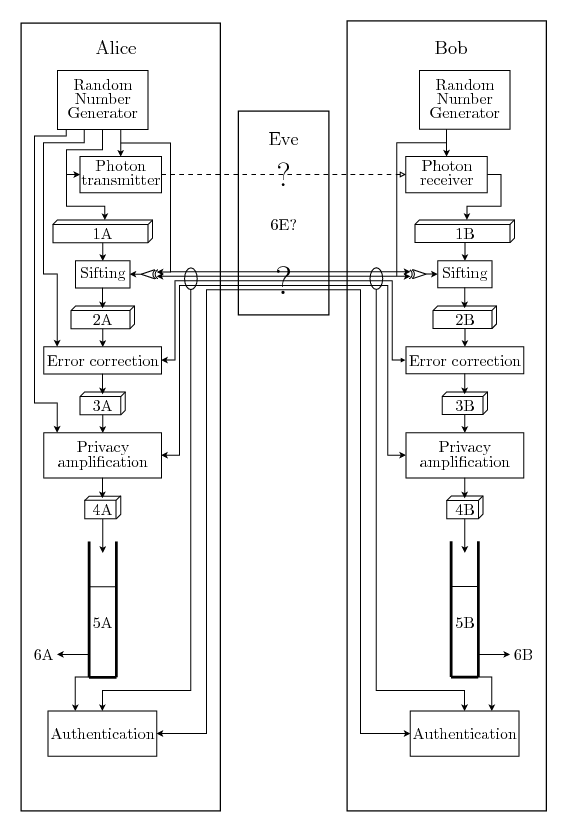
The QKG process is assumed to work in rounds, where each round consists of first using the quantum channel to transmit some photons and then using the classical channel to perform sifting, error correction, privacy amplification and authentication. During the authentication a piece of the shared key is used and destroyed, but if everything succeeds a larger piece can be added to the shared key.
In the BB84 protocol, the quantum transmission consists of
Alice trying to send lots of photons to Bob, where each photon is
transmitted in one of two bases, selected by the arrow that goes
into the top of the photon transmitter box in
figure 1.1. The photon also has
one of two values, selected by the arrow that enters the box from
the left, giving a total of four possible photon states. For
example, the two values in the first base can be represented by
horizontal and vertical polarization, while the two values in the
second base are represented by +45![]() and -45
and -45![]() polarization. She stores the values of all
photons sent in this round in 1A and
remembers the bases until the sifting
step.
polarization. She stores the values of all
photons sent in this round in 1A and
remembers the bases until the sifting
step.
Bob measures each received photon in a base randomly chosen from the same two bases, selected by the arrow at the top of the photon receiver box in the figure. If he used the same base as Alice and there were no transmission errors, the same value Alice used will come out on the right side of the box in the figure and be a part of 1B. It is important that those random choices are unpredictable. Quantum mechanics says that if Eve doesn't know the base of the photon she cannot copy a photon and resend it undisturbed. She can try to guess the base, but she has only a 50% chance to be correct, and if she is wrong she will only receive a random value and can not retransmit the photon to Bob undisturbed. If she introduces enough errors Alice and Bob will get suspicious, but there are always some errors on the channel anyway, so if Eve only makes some measurements the errors she introduces won't be seen behind the normal noise of the quantum channel. At least in theory she might even replace the optical fibre with a perfect photon channel, which gives her the possibility to introduce as many errors through measurements as the old fibre did by just being imperfect. Exactly what measurements she can make is the subject of much research, but for the current purposes it is sufficient to know that some information must be assumed to have leaked to her.
After the quantum transmission Alice and Bob will discuss over the classical channel what photons were received by Bob and which bases they both used. The values in 1A that Bob never received are discarded, as are the values in both 1A and 1B where Alice and Bob used different bases. This process is called sifting. When the sifting is done Alice and Bob will have the bit strings 2A and 2B, on average half the size of 1B and much smaller than 1A. Encrypting the sifting messages of one round would need much a much larger key than can be generated in one round, so they must be unencrypted and Eve will learn what bases Alice and Bob used. She will use that information to make better sense of whatever measurements she made on the quantum channel, but it is too late for her to base her measurements on that information. It is therefore important that Alice and Bob makes sure that the sifting is started after the quantum transmission is finished, e.g. by using synchronized clocks or by sending one random message from Alice to Bob, sending another from Bob to Alice and finally a third from Alice to Bob before starting the sifting, and authenticating those messages with the rest of the messages in the end of the round.
If the quantum channel was perfect and Eve didn't do anything the bit strings 2A and 2B would be identical. In practice the channel isn't perfect so the strings are not identical, but they are similar. By using the classical channel they can perform error correction and produce the shorter strings 3A and 3B which with very high probability are identical. If Eve has measured too much they will with very high probability notice that there are too many errors and abort.
Even though the errors were not alarmingly frequent Eve must be assumed to have made some measurements and will therefore know things about 3A and 3B. Alice and Bob therefore use the classical channel to perform privacy amplification. The result is the even shorter bit strings 4A and 4B which Eve with very high probability knows very little about. Unfortunately they can not remove her knowledge completely, but it can shrink quite fast for each bit they shorten their shared string with. As long as 4A and 4B are longer than the authentication keys needed the system will still create keys, but in a slower rate if the created strings are smaller.
After error correction and privacy amplification Alice and Bob have the bit strings 4A and 4B, and with very high probability those strings are both identical and unknown to Eve. At least if Eve has not interfered with their discussions over the classical channel. As an extreme example, Eve might have cut both cables and plugged in her own QKG system on the loose ends, playing the part of Bob when talking to Alice and the part of Alice when talking to Bob. This attack is generally known as a man-in-the-middle attack. But since Eve does not know the key generated previously or, if this is the first round, the key installed with the system, Alice and Bob can perform authentication of vital parts of their previous discussion using their shared key. If the authentication goes well, the generated key is considered secret and is added to the key storages 5A and 5B, ready to be used as authentication key later. The key streams 6A and 6B can be taken from 5A and 5B as long as there always is enough left to authenticate the next round. Those key streams are the whole point of the system.
If the authentication fails Eve is assumed to be trying to interfere and the process should be aborted. A complication is the fact that the error correction is not perfect. An error can, with a small probability, sneak through. If that error is in the key used for authentication in a later round, the authentication will fail even without an Eve being present.
If Eve somehow manages to break the security of one round she will know the authentication key for the next round and can break that too. No matter when she starts eavesdropping, if she breaks any round she therefore also breaks all future rounds. This problem might be partly possible to remedy, e.g. by making sure to always mix keys from several previous rounds to produce an authorization key, but research in that field is scarce.
2. QKG versus courier
A QKG system produces two identical secret key streams in two different places. A very old and reliable method to do the same thing is to simply have Alice generate a random secret in two copies and let a courier transfer one of them to Bob. Alice and Bob can then continuously read a secret key stream from their two copies while erasing whatever they read from their copies to minimize the risk of someone extracting their key streams later.
A QKG system can theoretically create key streams forever, but the whole courier carried secret will eventually be used and erased. If a never-ending key stream is required, a new courier will need to be sent whenever the last parts of the last secret is about to be used. How often that needs to be done depends on the required bit rate and how much each courier can carry. A famous quote from [5] goes Never underestimate the bandwidth of a station wagon full of tapes hurtling down the highway, often updated to more modern conditions as Never underestimate the bandwidth of a 747 filled with DVDs. However, with the limited range and bit rate of QKG systems, a courier carrying a hard disk by foot is enough to provide serious competition.
A courier is also needed for both the initial key and the QKG device in the QKG case. The difference in the pure courier method is that the initial key is made much larger and the device is neither transferred nor used. This chapter provides a comparison between a QKG system and a courier system.
2.1 Manufacturing and transferring
In both a QKG system and a courier system Alice needs to generate a random key to be copied and transferred to Bob. The courier system needs a larger key initially, which is a disadvantage. On the other hand, no QKG device needs to be manufactured and transferred. In addition, the amount of random data a QKG system needs when running is many times greater than the key it can produce, so the total amount of random data needed is much smaller in the courier case, but it needs to be available earlier.
The company IdQuantique which sells QKG systems also offers PCI card quantum random number generators capable of providing a 16 Mbit/s stream of random data to a normal computer, but much faster alternatives will surely surface if there is a high demand for them. An alternative to buying a random number generator is to buy the random numbers themselves. Companies may specialize in continuously manufacturing random secrets and selling them to customers. These companies would need to be trusted to not store copies of the secrets they generate and sell them to Eve, but even random number generators can, in theory, be manufactured to return a predictable number sequence so their manufacturers would also need to be trusted. When buying random numbers instead of random number generators, needing the random numbers early is no disadvantage since the sellers can be expected to have pregenerated numbers available. In any case, XORing the secrets from two or more companies makes the result secret even if only one of them is honest.
To transfer the initial key and device for the QKG system and the whole key in the courier system a trusted courier is needed. There is not much difference between a QKG system and a pure courier system in this step. In both cases, if Eve persuades or bribes the courier to show her or let her modify the key, Eve has won. The fact that the courier key is larger makes little difference. Eve will also win if she manages to rebuild the device, e.g. to include a backdoor accessible via radio or one of the channels, without Bob noticing. In both cases the trust in the courier can be enhanced with physical seals. The keys can also be made more safe by sending several different keys with different couriers and XORing the keys with each other to produce the real key. Eve will have to succeed in bribing every courier to get the key. However, they can't XOR physical devices, so Alice and Bob will have to set up and maintain as many QKG systems as they want couriers.
2.2 Unconditional security
QKG is often said to provide unconditional security. The security of most conventional cryptography is conditioned on the assumption that Eve's computational power and algorithms are limited. The security of QKG is not, hence the use of the term unconditional. This does not mean that the security of QKG is absolute or perfect. There exists many threats to a QKG system but, just as with a courier system, Eve having access to fast computers isn't one of them.
If the quantum channel is an optical fibre, Eve might be able to send light into the fibre to Alice's or Bob's device and gain information about the random settings from the reflected light. This attack is called a Trojan horse attack2.1 and QKG manufacturers do their best to protect their devices. Unfortunately, a perfect protection seems unlikely.
The classical channel is not without hazards either. In a typical scenario it is a network cable connecting two computers. The possibilities of cracking a computer if having access to a network cable are quite a few. Bugs in the computer software or in the network card might allow Eve to sneak by just sending the right information. By altering voltage levels she might be able to trigger just the right hardware failure that allows her full access. Even though the channel is built to be as secure as possible, perfect security is unattainable.
There are many other things that Eve can do that have a small but non-zero chance of succeeding. She can make many measurements on the quantum communication. If she is very lucky she will go undetected. She can also try to guess the authentication tags. The probability of her succeeding can be made very small, but it will always be there.
These examples have no counterpart in the courier system. There just is no communication necessary between Alice and Bob when their keys have been distributed. Lots of other attacks are still possible of course, such as infiltrating the building or bribing personnel, but those attacks are similar no matter what system is used.
2.3 Denial of Service attacks
The strength of QKG is that Alice and Bob can detect that Eve is attempting to intercept the key they are growing and allows them to abort. It does not guarantee that they can grow their key, and Eve can stop the key growing process at will. She might just cut the cables or she might deliberately make failed attempts to intercept, but Alice and Bob will not be able to grow their key when Eve won't let them. In reality, complicated systems tend to break even without deliberate sabotage so the key may stop growing even without Eve. The courier-only system does not have the problem of these kinds of deliberate Denial of Service attacks, and spontaneous failures should be far more rare due to the simplicity of the system. Other kinds of Denial of Service attacks are still possible, such as anything that physically destroys Alice's or Bob's device, but those attacks work on both the QKG system and the courier system.
2.4 Mobility
In the courier-only system Alice and Bob may move around freely and bring their keys. The QKG system is more stationary. It is hard to move devices connected through an underground cable. They must also be very close together, typically less than 100 km, and the bit rate decreases exponentially with the distance.
2.5 Time and price
A courier transmitted key can be used all at once or a little bit at a time, but when the whole key is used a new courier needs to be sent. A QKG generated key can not be used faster than it is generated, but it will in theory continue forever.
A 400 GB hard disk can today (2005) be bought for around 250 Euro. We can use one of those to store the courier key. If we use the high key rate of 1000 bits/s from [1], a QKG system can be replaced with this courier-delivered key and run for over 100 years before another courier needs to be sent. The prices of commercial QKG systems are unknown but are probably several hundred times more expensive than the hard disk. One would think that with such a saving and knowing that it provides better security, a courier delivering a new key once every century can be afforded. Especially since the distance is less than 100 km.
However, if the bit rates of the QKG systems grow faster than the sizes of cheap storage devices the couriers would have to run often enough that the QKG systems are cheaper when the limitations in stability, mobility and distance can be tolerated.
2.6
Limited lifetime
A QKG system with a limited lifetime will during that time produce a key as big as its key rate times its lifetime. Any such system can always be replaced by a courier system with a pregenerated key that big. Depending on what the future holds it might not necessarily be more cost effective, but the security is only affected positively. In practice everything can be expected to have a limited lifetime, but in Chapter 7 a weakness is identified that limits the lifetime of a QKG system even in theory. Fortunately, easy solutions to the problem exist and two of them are presented in the same chapter.
3. Discrete random variables
3.1 Discrete random variables
For the current purposes it is sufficient to think of a
discrete random variable ![]() as variable with a fixed but unknown integer
value larger than or equal to zero. The random variables we will
encounter later will be mostly secret keys, messages, and message
tags. Our knowledge about the random variable is completely
determined by a vector of positive probabilities
as variable with a fixed but unknown integer
value larger than or equal to zero. The random variables we will
encounter later will be mostly secret keys, messages, and message
tags. Our knowledge about the random variable is completely
determined by a vector of positive probabilities
![]() , each describing how
confident we are that the variable's value is the specific
integer
, each describing how
confident we are that the variable's value is the specific
integer ![]() , adding
up to 1. It is often better to talk about uncertainty, or
entropy, instead of knowledge. No uncertainty means full
knowledge, i.e., 100% probability for one value and 0% for the
rest.
, adding
up to 1. It is often better to talk about uncertainty, or
entropy, instead of knowledge. No uncertainty means full
knowledge, i.e., 100% probability for one value and 0% for the
rest.
An important special case is the random variables for which all non-zero probabilities are equal. These random variables are called uniform random variables. If Alice throws a normal, but perfect, six-sided die and keeps the result secret, the result is to Bob a uniform random variable with six possible values. If Bob had managed to replace Alice's die with one that is not perfect, the variable would not have been completely uniform. In any case, Alice knows the value so to her it is a random variable with zero uncertainty or entropy.
The range of ![]() is
the set of values
is
the set of values ![]() can
have, even those with zero probability, and is denoted
can
have, even those with zero probability, and is denoted
![]() . Even though
infinite ranges are possible, we will limit ourselves to random
variables with finite ranges. Without loss of generality we will
only consider ranges consisting of integers
. Even though
infinite ranges are possible, we will limit ourselves to random
variables with finite ranges. Without loss of generality we will
only consider ranges consisting of integers ![]() .
.
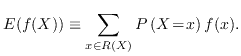
The expectation value is denoted ![]() and can be defined as
and can be defined as
Throughout the rest of this thesis the class of random
variables ![]() defined by (3.2) will serve as an
illustrative example. The same definition in Python code is
available as function Q in entropies.py line 54 .
defined by (3.2) will serve as an
illustrative example. The same definition in Python code is
available as function Q in entropies.py line 54 .
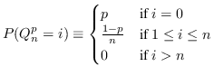
![]() is a uniform
random variable with
is a uniform
random variable with ![]() possible values. If
possible values. If ![]() is large
is large ![]() has one very probable and
has one very probable and
![]() equally
improbable values. Such random variables are rather extreme and
will therefore nicely illustrate some somewhat unintuitive
situations later.
equally
improbable values. Such random variables are rather extreme and
will therefore nicely illustrate some somewhat unintuitive
situations later.
3.2 Dependent random variables
Two random variables ![]() and
and ![]() can be related in ways that are unrelated to
their internal probability vectors. To completely specify both
their respective probability vectors and their relations it is
sufficient (and necessary) to (be able to) specify the
probability vector of a larger random variable, the concatenation of the two variables, written as
can be related in ways that are unrelated to
their internal probability vectors. To completely specify both
their respective probability vectors and their relations it is
sufficient (and necessary) to (be able to) specify the
probability vector of a larger random variable, the concatenation of the two variables, written as
![]() , with
probabilities
, with
probabilities
![]() and
and ![]() . Observe that neither
. Observe that neither ![]() nor
nor ![]() are products. When the random
variables are related in this way the probabilities in their
respective smaller probability vectors are called marginal probabilities.
are products. When the random
variables are related in this way the probabilities in their
respective smaller probability vectors are called marginal probabilities.
As an example, consider the dependent random variables defined by
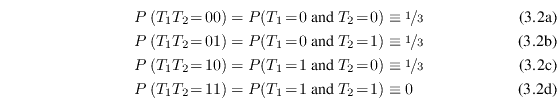
which can be seen as the two bits of the uniform random variable with values 0, 1 and 2. Their marginal distributions are
 |
Given two random variables ![]() and
and ![]() , when learning that the value of
, when learning that the value of
![]() is
is ![]() the probability vector of
the probability vector of
![]() can change. If
they are dependent
can change. If
they are dependent ![]() contains information about
contains information about ![]() and receiving information changes the
probabilities. The new random variable can be denoted
and receiving information changes the
probabilities. The new random variable can be denoted
![]() and
its probability vector is
and
its probability vector is
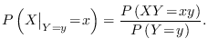
This relation is called Bayes' theorem and is a fundamental part of probability theory, but the notation is unorthodox.
Normally
![]() is written as
is written as
![]() and is read as
the probability that
and is read as
the probability that ![]() equals
equals ![]() given that
given that ![]() equals
equals ![]() . Similar notations are
used for other things, most notably for conditional entropy. We
will use the unconventional notation exclusively, both to note
explicitly that we are working on a new random variable and to
bring the implicit hidden expectation value in conditional
entropy written the conventional way out into the light. See
Chapter 4.4.1
for more details.
. Similar notations are
used for other things, most notably for conditional entropy. We
will use the unconventional notation exclusively, both to note
explicitly that we are working on a new random variable and to
bring the implicit hidden expectation value in conditional
entropy written the conventional way out into the light. See
Chapter 4.4.1
for more details.
Using Bayes' theorem on the previously defined ![]() and
and ![]() yields
yields
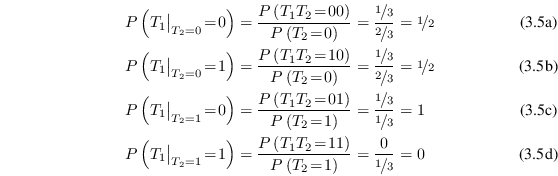 |
and, because of the symmetry in their definition, this also holds when
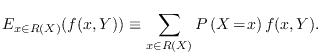
With more than one random variable it can be necessary to specify the expectation value over just one of them. A natural definition is
3.3 Jensen's inequality
There are lots of standard inequalities that are very useful in connection with random variables. We will only need one of them, Jensen's inequality.
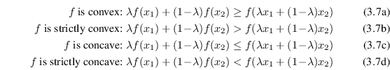
Jensen's inequality is applicable to convex and concave
functions. A function is called convex if it is continuous and
the whole line between every two points in its graph lies on or
above the graph. If the whole line lies above the graph it is
also called strictly convex. A function ![]() is concave3.1 or strictly concave if
is concave3.1 or strictly concave if ![]() is convex or strictly convex.
In other words, for all
is convex or strictly convex.
In other words, for all
![]() ,
,
![]() , and
, and
![]() holds:
holds:
 |
Jensen's inequality states that if
![]() is a convex or
concave function, then for any random variable
is a convex or
concave function, then for any random variable ![]() :
:
 |
Furthermore, if
For a random variable with only two possible values, Jensen's inequality just restates the definition of convexity. Generalizing to arbitrary number of values by induction is pretty straightforward and is explained in many other places.
If ![]() is
convex and has an inverse, an alternative way to express Jensen's
inequality is
is
convex and has an inverse, an alternative way to express Jensen's
inequality is
![]() .
.
4. Entropy
Entropy is an important concept in many fields, and one field where it is extensively used is QKG. This chapter gives a general overview of entropy and presents a generalization of the chain rule of entropy as needed in future chapters. Alternate explanations to most of the contents can be found in many other places, along with lots of other useful bounds and relations. The introductory chapters of [6] are highly recommended.
4.1 Conventions
The function
![]() where
where ![]() is a
probability occurs frequently in connection with entropies.
is a
probability occurs frequently in connection with entropies.
![]() is
normally undefined but since
is
normally undefined but since
![]() is well-defined we extend
the function to zero by continuity.
is well-defined we extend
the function to zero by continuity.
Another convention we will follow is to let
![]() mean
the logarithm base 2. We can choose any base, but using base 2
consequently means that everything will be expressed in bits, and
people tend to be familiar with bits.
mean
the logarithm base 2. We can choose any base, but using base 2
consequently means that everything will be expressed in bits, and
people tend to be familiar with bits.
4.2 Shannon entropy
Entropy is a measure of uncertainty regarding a discrete random variable. For many purposes, the Shannon entropy is the only measure needed. Shannon entropy is defined by
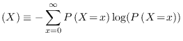
has the unit bits. A Python implementation is available as function shannon_entropy in entropies.py line 15 .
The Shannon entropy is a fundamental measure in information theory. It was introduced by Claude E. Shannon, now considered the father of information theory, in [7]. Much can be said about its properties, its uniqueness, and its relation with the thermodynamical entropy in physics, but we will only scratch a little bit on the surface here. One way of understanding it better is to rewrite the definition as
where
Now it is clear that the Shannon entropy is the expectation
value of ![]() where
where ![]() is the
probability assigned to the measured value of the random
variable.
is the
probability assigned to the measured value of the random
variable. ![]() can be interpreted as the needed length, in bits, of a message
communicating a measurement that had probability
can be interpreted as the needed length, in bits, of a message
communicating a measurement that had probability ![]() , which makes the Shannon entropy
a measure of the expected message length needed to communicate
the measured value of a random variable.
, which makes the Shannon entropy
a measure of the expected message length needed to communicate
the measured value of a random variable.
The Shannon entropy of a uniform random variable with
![]() possible values
is
possible values
is
| (4.3) |
which means that we need
Without qualifiers, the word entropy and a non-subscripted
![]() normally refers
only to Shannon entropy. However, when dealing with QKG, as well
as most other parts of cryptography, this measure is not
sufficient. The goal of QKG is to produce a key that is known to
both Alice and Bob but to Eve is a random variable with high
uncertainty.
normally refers
only to Shannon entropy. However, when dealing with QKG, as well
as most other parts of cryptography, this measure is not
sufficient. The goal of QKG is to produce a key that is known to
both Alice and Bob but to Eve is a random variable with high
uncertainty. ![]() is a measure of the uncertainty of a
value assigned probability
is a measure of the uncertainty of a
value assigned probability ![]() and is therefore a measure of the security of
that particular value of the key. Shannon entropy measures the
expectation value of that security. The dangers of focusing on
Shannon entropy alone is highlighted by this theorem:
and is therefore a measure of the security of
that particular value of the key. Shannon entropy measures the
expectation value of that security. The dangers of focusing on
Shannon entropy alone is highlighted by this theorem:
 |
(4.4) |
which completes the proof. ![]()
Good security average is not good enough, and Shannon entropy alone is obviously not a sufficient measure of the quality of a key.
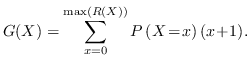
4.3 Guessing entropy
Another measure more closely related to the difficulty of
guessing the value of a random variable was introduced by Massey
in [8]. He did not name it but in
[6] it is called guessing entropy. Note, however, that while most
other entropies have the unit bits
the guessing entropy is measured in units of number of guesses. Without loss of generality we
can assume that the values of ![]() are sorted with decreasing probability, in which
case the guessing entropy of
are sorted with decreasing probability, in which
case the guessing entropy of ![]() is defined as
is defined as
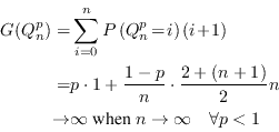
That is, the guessing entropy is simply the average number of guesses needed to guess the value of a random variable using the optimal strategy. The definition formalized to Python code is available as function guessing_entropy in entropies.py line 36 . We have yet again a measure of average security and similarly to theorem 1 we can write
 |
(4.6) |
which completes the proof.
Again we see that good security average is not good enough, and guessing entropy alone is not a sufficient measure of the quality of a key.
4.4 Rényi entropy
A useful generalization of Shannon entropy is the Rényi
entropy, which maps an entropy measure
![]() pronounced the Rényi entropy of order
pronounced the Rényi entropy of order
![]() to
every real number
to
every real number
![]() . Rényi entropy is, just
like Shannon entropy, measured in units of bits.
. Rényi entropy is, just
like Shannon entropy, measured in units of bits.
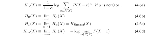
The equality in (4.7c) is easy to show using e.g. l'Hospital's4.2 rule. The definition is also available as Python code as function entropy in entropies.py line 23 .
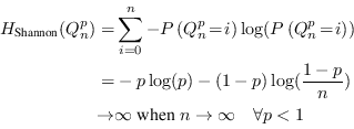
An important property of Rényi entropy is that for
![]() ,
,
![]() for all
for all
![]() , with equality if
and only if
, with equality if
and only if ![]() is a
uniform random variable. In other words,
is a
uniform random variable. In other words,
![]() is a
constant function of
is a
constant function of ![]() if
if ![]() is uniform and strictly decreasing if not. A
full proof is given in [6] and follows
quite naturally by writing
is uniform and strictly decreasing if not. A
full proof is given in [6] and follows
quite naturally by writing
![]() in
analogy with (4.2) as
in
analogy with (4.2) as
![]() and using Jensen's inequality.
and using Jensen's inequality.
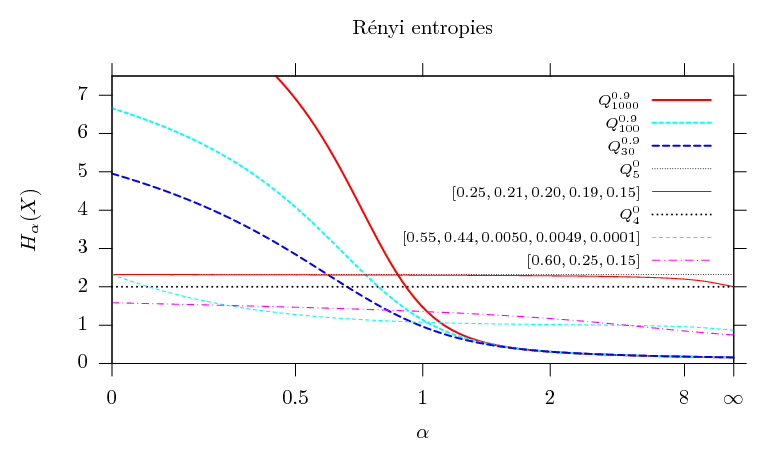
Some of these measures have quite natural interpretations.
Rényi entropies with higher ![]() parameter depend more on the probabilities
of the more probable values and less on the more improbable ones.
parameter depend more on the probabilities
of the more probable values and less on the more improbable ones.
![]() is logarithm
of the number of values of
is logarithm
of the number of values of ![]() that have non-zero probabilities. Any two random
variables with different probability distributions but the same
number of values with non-zero probabilities will have the same
Rényi entropy of order 0.
that have non-zero probabilities. Any two random
variables with different probability distributions but the same
number of values with non-zero probabilities will have the same
Rényi entropy of order 0.
![]() is the
Shannon entropy, in which the actual probabilities are quite
important.
is the
Shannon entropy, in which the actual probabilities are quite
important.
![]() is often
called collision entropy, or just Rényi entropy, and is the
negative logarithm of the likelihood of two independent random
variables with the same probability distribution to have the same
value. More probable values are much more likely to collide and
are therefore more visible in the collision entropy than in the
Shannon entropy.
is often
called collision entropy, or just Rényi entropy, and is the
negative logarithm of the likelihood of two independent random
variables with the same probability distribution to have the same
value. More probable values are much more likely to collide and
are therefore more visible in the collision entropy than in the
Shannon entropy.
![]() is
called min-entropy and is a function of the highest probability
only.
is
called min-entropy and is a function of the highest probability
only.
The shape of
![]() as a
function of
as a
function of ![]() for
eight different random variables
for
eight different random variables ![]() is shown in figure 4.1.
is shown in figure 4.1.
4.4.1 Conditional
Rényi entropy
The conditional
Shannon entropy for It expresses the expected value of the entropy of
 |
(4.9) |
which is a single expectation value just like equation (4.2).
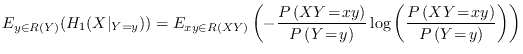
Rényi entropies of different order than 1 are not
expectation values so things are not quite as simple. In fact,
according to [6] there is not even an
agreement about a standard definition of conditional Rényi
entropy. However, the dominant definition seems to be the same as
(4.8) with both ![]() :s replaced by
:s replaced by ![]() . That definition will be
used here but the expectation value will always be explicitly
written out. We have seen that averaging security can be
dangerous, and it is nice to not hide away something potentially
dangerous in the notation.
. That definition will be
used here but the expectation value will always be explicitly
written out. We have seen that averaging security can be
dangerous, and it is nice to not hide away something potentially
dangerous in the notation.
4.4.2 Chain rule of Rényi entropy
With conditional Shannon entropy comes the chain rule of Shannon entropy, equation (4.10b) below. One way to define conditional Rényi entropy is to choose it so the same relation still holds when the Shannon entropies are replaced with Rényi entropies. However, the relation does not hold for the expectation value based definition chosen above so it is clearly a different conditional entropy. Fortunately, that doesn't stop us from generalizing the chain rule in other ways to something that is useful with general Rényi entropies:
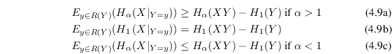
with equality in (4.10a) and (4.10c) if and only if
 |
(4.11) |
When ![]() we have instead:
we have instead:
 |
(4.12) |
The function
4.4.3 Spoiling knowledge
When learning something new about a random variable, the
Shannon entropy of the variable will decrease or stay equal on
average. It is only true on average. Consider
![]() and a
and a ![]() that is
dependent on
that is
dependent on ![]() such that
such that ![]() if
if
![]() and
and
![]() if not.
Learning that
if not.
Learning that ![]() is
1 will increase the Shannon entropy of
is
1 will increase the Shannon entropy of ![]() from 0.15 to 6.64, but learning
that
from 0.15 to 6.64, but learning
that ![]() is 0
will decrease it to exactly 0. On average, the Shannon entropy
will decrease to 0.0664. On average, the Shannon entropy will
always decrease for all
is 0
will decrease it to exactly 0. On average, the Shannon entropy
will decrease to 0.0664. On average, the Shannon entropy will
always decrease for all ![]() and
and ![]() .
.
However, that is not true in general for other Rényi
entropies. For example, consider ![]() and
and ![]() defined in (3.3a).
defined in (3.3a).
![]() . If
. If
![]() turns out to be
1 the entropy of
turns out to be
1 the entropy of ![]() reduces to exactly 0, if not it becomes exactly 1. On average, it
will increase to
reduces to exactly 0, if not it becomes exactly 1. On average, it
will increase to
![]() .
.
Side information that increases entropy on average like this was first mentioned in [9] and is called spoiling knowledge.
4.4.4 Entropy holism
The Concise Oxford English Dictionary [10] describes holism as the
theory that certain wholes are greater than the sum of their
parts. In a way, random variables normally behave in a
holistic way. To specify both ![]() and
and ![]() the whole probability vector for
the whole probability vector for ![]() is needed and the size of
is needed and the size of
![]() is the size
of
is the size
of ![]() multiplied by
the size of
multiplied by
the size of ![]() .
This is one reason why Shannon chose to primarily use a
logarithmic scale in [7]. With a
logarithmic scale the multiplications can be treated as sums and
the whole is just the sum of the parts. Quoting Shannon:
One feels, for example, that two punched
cards4.3 should
have twice the capacity of one for information storage, and two
identical channels twice the capacity of one for transmitting
information.
.
This is one reason why Shannon chose to primarily use a
logarithmic scale in [7]. With a
logarithmic scale the multiplications can be treated as sums and
the whole is just the sum of the parts. Quoting Shannon:
One feels, for example, that two punched
cards4.3 should
have twice the capacity of one for information storage, and two
identical channels twice the capacity of one for transmitting
information.
It should come as no surprise that an important property of Shannon entropy is that the total entropy of a system is never greater than the sum of the parts' entropies,
where
On the other hand, what might come as a surprise is that this
is not true in general for other Rényi entropies. There
exists ![]() and
and
![]() such
that
such
that
For example, consider ![]() and
and ![]() defined in (3.3a)
again.
defined in (3.3a)
again.
![]() but
but
![]() .
This is a case where the whole actually is greater than the sum
of the parts.
.
This is a case where the whole actually is greater than the sum
of the parts.
5. Unconditionally secure
authentication
The two most important areas of cryptography are encryption and authentication - making sure that no one except the legitimate receiver reads the message and making sure that nobody except the legitimate sender writes or modifies it. A typical encryption scenario is Alice wanting to send Bob a secret message, but instead of sending the message directly she sends something that Bob can transform to the real message but which means nothing to anyone else. A typical authentication scenario is Alice sending Bob a message which Bob wants to be sure originates from Alice and nobody else. Alice sends the message as-is but also attaches a tag5.1, a few bytes large, which depends on the message. Typically only one tag is valid for each possible message and nobody except Alice and Bob5.2, knows beforehand which one. When Bob has received both the message and the tag he can verify that the tag is correct and conclude that the message really originated from Alice, or at least someone with access to Alice's key, and has not been tampered with on the way to him.
Whenever encryption is explained the one-time pad encryption, commonly referred to as
simply OTP, almost always serves as
an enlightening example. OTP was co-invented in 1917 by Gilbert
Vernam and Major Joseph Mauborgne (see e.g. [11]) and and in the 40's Claude
Shannon proved both that it was unbreakable and that any
unbreakable encryption is essentially equivalent to OTP. The
encryption is very simple. For Alice to send Bob a message
![]() they need to
share a secret completely random key
they need to
share a secret completely random key ![]() , the one-time pad, which needs
to be at least as long as the message and must never be reused.
Alice simply sends
, the one-time pad, which needs
to be at least as long as the message and must never be reused.
Alice simply sends
![]() XOR
XOR ![]() and Bob
calculates
and Bob
calculates
![]() XOR
XOR ![]() XOR
XOR ![]() .5.3 OTP is
almost never used in practice. There exists many other encryption
schemes that require smaller keys, don't require a key known by
both Alice and Bob and permits reusing of keys. They are all
theoretically breakable given enough computation power or maybe
good enough algorithms, but are by most regarded secure enough.
OTP serves mainly as an example.
.5.3 OTP is
almost never used in practice. There exists many other encryption
schemes that require smaller keys, don't require a key known by
both Alice and Bob and permits reusing of keys. They are all
theoretically breakable given enough computation power or maybe
good enough algorithms, but are by most regarded secure enough.
OTP serves mainly as an example.
Even though OTP is universally known for providing unbreakable encryption, few know that something similar exists for authentication. It was invented in the late 70's by J. Lawrence Carter and Mark N. Wegman who published their discoveries in [12] and [13]. It is commonly referred to as Wegman-Carter (type) authentication. One can only speculate why it is almost completely unheard of in the popular science , but contributing factors are surely that it is much newer than OTP, that it is much more complicated to explain and that authentication itself is more complicated and often regarded as less interesting. Furthermore, one example of unbreakability is maybe enough for most purposes. On top of that, if something is encrypted with OTP it is impossible to extract any information at all about the message, but with any authentication scheme it is always possible for Eve to produce a random tag and hope it is the correct one for the message she wants to make Bob believe Alice has sent. The best that can be done for authentication is to make the probability that Eve succeeds arbitrarily small, and that is exactly what Wegman-Carter authentication does.
The main problem with OTP is that the required key needs to be at least as long as the message to be encrypted. Wegman-Carter authentication does not share this problem. The keys can be much shorter, in the order of a few bytes. The fact that the required keys can be much shorter than the message to be authenticated is essential for QKG. Each round of a QKG protocol generates a certain amount of shared secret key and requires far more communication which needs to be authenticated. If the key consumed by the authentication process is larger than the generated key we don't have Quantum Key Growing but Quantum Key Shrinking which would be quite pointless.
Other authentication methods exist where instead of just one tag being sent from Alice to Bob a dialogue is held with several messages going back and forth. They can be more effective in terms of consumed key but are not necessary for QKG and are beyond the scope of this work. This chapter describes unconditionally secure message authentication in the theoretical scenario where Alice and Bob share a completely secret key and wish to transmit an unmodified message through a channel completely controlled by Eve, not necessarily as part of a QKG system. In the next chapter the authentication is made more realistic for a QKG scenario by assuming that the key is not completely secret, and in Chapter 7 everything is put into a QKG context.
5.1 Universal families of hash functions
A very useful tool in cryptography is the concept of cryptographically secure hash functions. Unfortunately, like most cryptography used in the real world they are only secure against what is believed to be practical attacks and can be broken with enough computation power or, if they exist, good enough algorithms. It is impossible to construct an unbreakable cryptographically secure hash function. See e.g. [14] for definitions and proofs.
Cryptographically secure hash functions can be used for many things, one of them being message authentication. Although hash functions cannot be unbreakable, message authentication can. A word of warning is in place here regarding terminology. The fundamental building block of the unbreakable Wegman-Carter authentication is called universal families5.4 of hash functions, but those hash functions are quite different from the cryptographically secure hash functions mentioned above. They have similarities and both deserve to be called hash functions, but the individual hash functions of Wegman-Carter are not, and need not be, cryptographically secure in the classical sense.
Families of hash functions can be used for many things and
many different requirements can be put on them. A system has
evolved to express the requirements a family fulfills. For
authentication a definition of ![]() -almost
strongly-universal
-almost
strongly-universal![]() (
(![]() -ASU
-ASU![]() ) is sufficient. Wegman
and Carter began with a stronger requirement in [12] but the keys needed to be far too big for
authentication to be practical. In [13] they
showed that by loosening the requirements somewhat the
authentication can still be acceptably secure but the required
length of the keys shrinks considerably. Although they defined
similar requirements and presented an example of an
) is sufficient. Wegman
and Carter began with a stronger requirement in [12] but the keys needed to be far too big for
authentication to be practical. In [13] they
showed that by loosening the requirements somewhat the
authentication can still be acceptably secure but the required
length of the keys shrinks considerably. Although they defined
similar requirements and presented an example of an ![]() -almost
strongly-universal
-almost
strongly-universal![]() family, they gave it no formal definition. The first formal
definition appeared in [15].
family, they gave it no formal definition. The first formal
definition appeared in [15].
- (a)
- The number of hash functions in
 that takes an arbitrary
 to an arbitrary
 is exactly
 .
. - (b)
- The fraction of those functions that also takes an
arbitrary
 in
in
 to
an arbitrary
to
an arbitrary
 (possibly equal to
 ) is no
more than
) is no
more than  .
.
Note that it is not possible to have an
![]() .
The special case
.
The special case
![]() was
the unnecessarily strong requirement in [12]
and those families are simply called strongly universal
was
the unnecessarily strong requirement in [12]
and those families are simply called strongly universal![]() (SU
(SU![]() ). In theory
). In theory ![]() can be as large as 1,
but in practice the family will not be of much use unless
can be as large as 1,
but in practice the family will not be of much use unless
![]() is rather
close to
is rather
close to
![]() . One example of
a 1-almost strongly-universal
. One example of
a 1-almost strongly-universal![]() family is the
family is the
![]() hash functions simply
defined as
hash functions simply
defined as
![]() , where
, where
![]() is the
modulo operation from computing, the remainder after division,
rather than the modular arithmetic of algebra. The number of hash
functions is equal to the number of tags, but a message/tag pair
uniquely identifies the hash function which makes the family
unsuitable for use in authentication.
is the
modulo operation from computing, the remainder after division,
rather than the modular arithmetic of algebra. The number of hash
functions is equal to the number of tags, but a message/tag pair
uniquely identifies the hash function which makes the family
unsuitable for use in authentication.
Note also that the number of hash functions in the family must
be at least
![]() , so the
key needed to specify a member of the family must be larger than
the generated tag.
, so the
key needed to specify a member of the family must be larger than
the generated tag.
A strongly universal![]() family is in computer science often called
pairwise independent family of hash
functions. When hashing two distinct messages using the
same random hash function, the two resulting tags are
statistically independent. This is the significance of the number
2 in the subscript. Note that even though a set of random
variables are pairwise independent, they are not necessarily
mutually independent or even 3-wise independent. In general, a
strongly universal
family is in computer science often called
pairwise independent family of hash
functions. When hashing two distinct messages using the
same random hash function, the two resulting tags are
statistically independent. This is the significance of the number
2 in the subscript. Note that even though a set of random
variables are pairwise independent, they are not necessarily
mutually independent or even 3-wise independent. In general, a
strongly universal![]() family is the same thing a
family is the same thing a ![]() -wise independent family and means that all sets
of
-wise independent family and means that all sets
of ![]() distinct
messages are mapped to statistically independent tags, which is a
stronger condition for higher
distinct
messages are mapped to statistically independent tags, which is a
stronger condition for higher ![]() .
.
5.2
Examples
Wegman and Carter proposed several strongly
universal![]() families
in [12] and one
families
in [12] and one
![]() -almost
strongly universal
-almost
strongly universal![]() in
[13]. The hash families of Wegman-Carter are
by no means unique or most effective, but since they are the
original ones they are both interesting from a historical point
of view and are often referenced. Furthermore, they are quite
easy to understand and their performance is, although not
optimal, good enough for many examples and applications.
in
[13]. The hash families of Wegman-Carter are
by no means unique or most effective, but since they are the
original ones they are both interesting from a historical point
of view and are often referenced. Furthermore, they are quite
easy to understand and their performance is, although not
optimal, good enough for many examples and applications.
One of the families they described is a simple strongly
universal![]() family
they called
family
they called ![]() .
Actually, the family is not really strongly universal
.
Actually, the family is not really strongly universal![]() . It is however ``close'' (their
quotation marks) and they treat it as if it was strongly
universal
. It is however ``close'' (their
quotation marks) and they treat it as if it was strongly
universal![]() . We will
do the same.
. We will
do the same.
An implementation of the family is available as function
H1 in hashfunctions.py line
85 . In words, the
family of hash functions mapping a message
![]() to a tag
to a tag
![]() needs a key consisting of
three parts. The first part is any prime number
needs a key consisting of
three parts. The first part is any prime number
![]() and
need not be secret. The other two parts are two secret integers
and
need not be secret. The other two parts are two secret integers
![]() and
and
![]() . The hash function defined by
this key simply maps a message
. The hash function defined by
this key simply maps a message ![]() to a hash value
to a hash value
![]() . As Wegman and Carter
write in [13], this can be generalized using
all polynomials of degree5.5 less than 2 over any Galois field,
and if the size of the Galois field is divisible with the number
of possible tags the family is strongly universal
. As Wegman and Carter
write in [13], this can be generalized using
all polynomials of degree5.5 less than 2 over any Galois field,
and if the size of the Galois field is divisible with the number
of possible tags the family is strongly universal![]() . If not, the mapping from the
field to a tag,
. If not, the mapping from the
field to a tag, ![]() above, will favor the lower tags
somewhat. In our case the size of the field is always a prime
number and larger than the highest message, so unless the tags
can be larger than the message the mapping can not be perfect,
but will be quite close.
above, will favor the lower tags
somewhat. In our case the size of the field is always a prime
number and larger than the highest message, so unless the tags
can be larger than the message the mapping can not be perfect,
but will be quite close.
The secret key needed to select a hash function from this family needs to be very big, roughly twice as big as the message to be hashed. A QKG system could never work using this family as authentication. The traffic that needs authentication each round is much larger than the generated key, so the shared secret key would shrink. The next family is not quite as secure but the probability of guessing a tag is at most doubled and the required key size grows much slower than the message size.
|
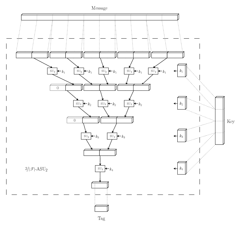
This
![]() -almost
strongly universal
-almost
strongly universal![]() family works by picking several hash functions from a much
smaller but strongly universal
family works by picking several hash functions from a much
smaller but strongly universal![]() family and applying them in a hierarchical
manner. Let the smaller family consist of hash functions mapping
bit strings of length
family and applying them in a hierarchical
manner. Let the smaller family consist of hash functions mapping
bit strings of length ![]() to bit strings of length
to bit strings of length ![]() , where
, where ![]() is slightly larger than the
length of the tag we want to produce. Divide the message into
substrings of length
is slightly larger than the
length of the tag we want to produce. Divide the message into
substrings of length ![]() , padding the last substring with zeroes if
necessary. Pick a hash function from the small family, apply that
function to each of the substrings and concatenate the results.
Repeat until only one substring of length
, padding the last substring with zeroes if
necessary. Pick a hash function from the small family, apply that
function to each of the substrings and concatenate the results.
Repeat until only one substring of length ![]() is left, using a new hash
function each repetition. Discard the most significant bits that
won't fit into the tag. What is left is the final tag.
is left, using a new hash
function each repetition. Discard the most significant bits that
won't fit into the tag. What is left is the final tag.
One round of hashing halves the length of the message, regardless of its size, but uses only one hash function, and only one small key to pick that hash function. The total key length needed therefore grows with approximately the logarithm of the message length. This means a QKG system can always be designed with large enough rounds to make the key used for authentication acceptably small in comparison to the created shared secret.
For the full details of this family, see either [13] or the Python implementation function
Hprime in hashfunctions.py
line 123 . For
an implementation using that function together with the strongly
universal![]() from the
previous example, see function Hprime_H1 in hashfunctions.py line 186 . A
functionally equivalent but more compact implementation of the
same function that might be easier to get an overview of, at the
expense of not following the Wegman-Carter papers as closely, is
available at function Hprime_H1_compact in hashfunctions.py line 214 .
from the
previous example, see function Hprime_H1 in hashfunctions.py line 186 . A
functionally equivalent but more compact implementation of the
same function that might be easier to get an overview of, at the
expense of not following the Wegman-Carter papers as closely, is
available at function Hprime_H1_compact in hashfunctions.py line 214 .
5.3
Authentication
Any Now suppose Eve has control over the channel between Alice and
Bob and wants Bob to accept a faked message
![]() .
To her the secret key is a random variable
.
To her the secret key is a random variable ![]() uniform over its whole range
uniform over its whole range
![]() . If the key is a
random variable, so is the correct tag
. If the key is a
random variable, so is the correct tag
![]() . The
first condition of definition 1
says that if
. The
first condition of definition 1
says that if ![]() is uniform over its whole range, so is
is uniform over its whole range, so is ![]() . She can take a guess, but any
guess has probability
. She can take a guess, but any
guess has probability
![]() to be
correct.
to be
correct.
She may also wait until Alice tries to send an authenticated
message to Bob, pick up the message and the tag, and make sure
Bob never see them. With both ![]() and
and
![]() at
her disposal she can, given enough computing power, rule out all
keys that do not match and be left with just
at
her disposal she can, given enough computing power, rule out all
keys that do not match and be left with just
![]() of the keys to
guess from. However, the second condition of
definition 1 says that even
with this knowledge she has, with
of the keys to
guess from. However, the second condition of
definition 1 says that even
with this knowledge she has, with ![]() uniform over its whole range, at best the
probability
uniform over its whole range, at best the
probability ![]() to guess the correct tag
to guess the correct tag ![]() for any
for any
![]() .
.
![]() is never
smaller than
is never
smaller than
![]() so
so ![]() is clearly an upper
limit on the probability that Eve makes the right guess and
manages to fool Bob into accepting a fake message, at least if
Eve knows nothing about the key beforehand.
is clearly an upper
limit on the probability that Eve makes the right guess and
manages to fool Bob into accepting a fake message, at least if
Eve knows nothing about the key beforehand.
5.4
Encrypted tags
If the same key is used twice for authentication, the
definition of ![]() -almost strongly-universal
-almost strongly-universal![]() families makes no guarantees
about how hard it is to guess the correct tag corresponding to a
third message. The keys must therefore never be reused. For each
authenticated message, Alice and Bob must sacrifice
families makes no guarantees
about how hard it is to guess the correct tag corresponding to a
third message. The keys must therefore never be reused. For each
authenticated message, Alice and Bob must sacrifice
![]() bits of their shared secret. Wegman and Carter describes in
chapter 4 in [13] a method of sacrificing
only
bits of their shared secret. Wegman and Carter describes in
chapter 4 in [13] a method of sacrificing
only
![]() bits for each message.
Begin by choosing a hash function
bits for each message.
Begin by choosing a hash function ![]() randomly from an
randomly from an ![]() -almost strongly-universal
-almost strongly-universal![]() family. This hash function will
be used for all messages, but the tag is calculated as
family. This hash function will
be used for all messages, but the tag is calculated as
![]() XOR
XOR ![]() . In other words,
the tag is one-time pad encrypted using the one-time pad
. In other words,
the tag is one-time pad encrypted using the one-time pad
![]() the same size as
the tag.
the same size as
the tag.
If ![]() is
is ![]() -almost
strongly-universal
-almost
strongly-universal![]() ,
so is
,
so is
![]() XOR
XOR ![]() . The
key, secret or not, merely reorders the tags which has no effect
on definition 1. Eve's chance
to guess the tag is therefore still limited by
. The
key, secret or not, merely reorders the tags which has no effect
on definition 1. Eve's chance
to guess the tag is therefore still limited by ![]() . The one-time pad
encryption makes sure no information about the hash function
leaks to Eve, so the hash function can be safely reused an
arbitrary number of times as long as new one-time pads are used
each time.
. The one-time pad
encryption makes sure no information about the hash function
leaks to Eve, so the hash function can be safely reused an
arbitrary number of times as long as new one-time pads are used
each time.
To authenticate the first message both a hash function and a one-time pad needs to be chosen so the required key is larger than in the authentication described above. However, each message after the first needs just a key of the same size as the tag, so the average sacrificed key length per message will approach the size of the tag.
6. Authentication with partially
secret key
In the previous chapter we assumed that Eve had no information
on the secret key used in the authentication, i.e., to Eve the
key ![]() was a random
variable uniform over its whole range. As explained in
Section 1.2 that is an
unrealistic requirement in QKG. Information leakage in the
quantum transmission phase is unavoidable but the damage can be
reduced using privacy amplification. Through the privacy
amplification process Eve's knowledge of the key is reduced, but
not to exactly zero. As soon as the whole initial key is used
Alice and Bob will have to start trusting authentication with a
key that is not completely secret. This chapter deals with
authentication with a partially secret key in general, while the
next chapter puts the results into the context of QKG.
was a random
variable uniform over its whole range. As explained in
Section 1.2 that is an
unrealistic requirement in QKG. Information leakage in the
quantum transmission phase is unavoidable but the damage can be
reduced using privacy amplification. Through the privacy
amplification process Eve's knowledge of the key is reduced, but
not to exactly zero. As soon as the whole initial key is used
Alice and Bob will have to start trusting authentication with a
key that is not completely secret. This chapter deals with
authentication with a partially secret key in general, while the
next chapter puts the results into the context of QKG.
If Eve holds some information about the authentication key, her chance of forgery may be much higher for some messages than others. For example, imagine Alice and Bob are authenticating messages using the second hash family in Section 5.2. Remember that those hash functions works by applying a number of smaller hash functions, each hash function halving the length of the message. If Eve knows the first hash function with certainty but nothing else and sees a valid message/tag pair from Alice, she can divide the message into substrings and change each substring to another that yields the same hash after the first step. No matter what the other hash functions are, the fact that the internal state after the first step is the same guarantees that the same tag is produced. However, if she wants to forge another message she is not helped at all by knowing the first hash function. But that is a weak comfort for Alice and Bob. Their goal was for Bob to verify that exactly the message he received was sent by Alice. No matter how limited Eve's choices are when choosing a forged message, Alice and Bob have failed if Eve makes any undetected change to the message. To be on the safe side we will consider the possibility of Eve to make an undetected change at all, without being bothered with how happy she is with the choice of message.
6.1 Active and passive chance of forgery
Eve's main goal is to make Bob accept a fake message, but her secondary goal is to avoid raising suspicions if she fails. If she has the possibility to first perform passive eavesdropping on the message and tag sent by Alice, and then decide whether she will launch a full-fledged active attack and send a forged message to Bob, it makes sense to divide Eve's chance of forgery into a passive part and an active part.
We can number the different states that Eve may be in after
the eavesdropping phase depending on what message/tag pair she
sees, denote the probability that she is in state ![]() with
with
![]() and the probability that an active attack succeeds if she chooses
to launch one with
and the probability that an active attack succeeds if she chooses
to launch one with
![]() . Her total chance of succeeding
is
. Her total chance of succeeding
is
| (6.1) |
As long as Eve stays passive she does not risk detection, but
if she chooses to make an active attack the chance of success is
![]() depending on the state she is in. If she fails to guess the tag
correctly she is detected when Bob notices that it does not match
the message. We will see that this difference between Eve's total
and active chance of forgery is especially important in QKG and
in other scenarios where many messages are sent and Eve only
needs to forge one of them.
depending on the state she is in. If she fails to guess the tag
correctly she is detected when Bob notices that it does not match
the message. We will see that this difference between Eve's total
and active chance of forgery is especially important in QKG and
in other scenarios where many messages are sent and Eve only
needs to forge one of them.
If Eve just needs to forge one message from an infinite stream
of messages, she will wait until she after the eavesdropping
phase is in the state with highest probability to guess a correct
tag. As long as the passive probability for that state is
non-zero, the probability that she will sometime reach that state
will go to 1 as the number of messages goes to infinity, and
Eve's chance of having forged a message will approach
![]() . If
. If
![]() is not acceptably
small, Alice and Bob must be prepared for the day when Eve
succeeds.
is not acceptably
small, Alice and Bob must be prepared for the day when Eve
succeeds.
6.2 No message/tag pairs seen
Eve doesn't need to know the whole key to be able to forge a message without any risk of being discovered, even when she cannot see a valid message/tag pair. The key is always larger than the tag and Eve needs only as much information that is contained in the tag. In other words, there are many hash functions that takes a single message to the same tag, and if her uncertainty about the key just makes her incapable of knowing which of those hash functions is used she still knows the correct tag with certainty. On the other hand, any information that just helps her pinpoint the exact hash function within the subsets that maps her message to the same tags is quite worthless.
Fortunately for Eve, what is worthless key information when
trying to forge one message need not be when trying to forge
another. The first condition of definition 1 states that exactly
![]() keys or hash functions take a single message to a single tag. The
second condition implies that the grouping of keys is different
for each message. A natural upper bound for Eve's active chance
to forge any message is therefore the sum of probabilities for
the
keys or hash functions take a single message to a single tag. The
second condition implies that the grouping of keys is different
for each message. A natural upper bound for Eve's active chance
to forge any message is therefore the sum of probabilities for
the
![]() most probable keys. The min-entropy of the key,
most probable keys. The min-entropy of the key,
![]() , is
the negative logarithm of the highest probability so if we let
, is
the negative logarithm of the highest probability so if we let
![]() denote the key
length in bits and
denote the key
length in bits and ![]() the tag length, a somewhat looser but simpler bound is given
by
the tag length, a somewhat looser but simpler bound is given
by
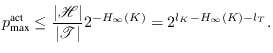 |
(6.2) |
If Eve knows nothing about the key her key (min-)entropy
equals the size of the key and chance is bounded by ![]() as expected.
as expected.
6.3 Encrypted tags
The method of one-time pad encryption of the tag described in
(5.4) makes authentication of a
constant stream of messages cheap and works fine when completely
secret one-time pads are available. However, when the one-time
pads are not guaranteed to be completely secret, Eve will learn
something about the hash function for each message/tag pair she
sees. The information she has about the one-time pad ![]() will equal the knowledge she
gains about
will equal the knowledge she
gains about ![]() when
she sees
when
she sees ![]() and
and
![]() XOR
XOR ![]() .
.
If Eve is unlucky she will only gain information she already
had. The exact knowledge of ![]() she gains depends not only on her exact
knowledge of
she gains depends not only on her exact
knowledge of ![]() but also on
but also on ![]() , so
it is very hard to put restrictions only on Eve's knowledge that
guarantees that she does not learn anything new.
, so
it is very hard to put restrictions only on Eve's knowledge that
guarantees that she does not learn anything new.
All Eve has to do to exploit this weakness is to passively eavesdrop the messages and the encrypted tags and combine that information with whatever she knows about the one-time pads until she has enough confidence in her knowledge of the hash function that she can mount an attack that succeeds with acceptable probability. In other words, her active chance of forgery will increase for (almost) each message/tag pair she sees if encrypted tags are used. Therefore, using the encrypted tags method is not advisable unless the one-time pads are known to be completely secret. Using the normal method of selecting a new hash function for each message does not share this problem.
6.4 A message/tag pair seen
If Eve sees a message/tag pair from Alice to Bob she is given
information about the authentication key, and she will combine
that information with whatever she knew about the key initially.
We will call the initial key before she has seen the tag
![]() and the key it
reduces to after the tag
and the key it
reduces to after the tag ![]() is revealed
is revealed
![]() .
.
The change of her uncertainty about the key when she sees the
tag is quite simple. The
![]() keys consistent with the message/tag pair seen are singled out
and normalized and the rest are set to 0. A limit for the average
Rényi entropy of order 1 or larger of the resulting key is
given by theorem 3,
keys consistent with the message/tag pair seen are singled out
and normalized and the rest are set to 0. A limit for the average
Rényi entropy of order 1 or larger of the resulting key is
given by theorem 3,
| (6.3) |
This is only a limit on the expectation value of the entropy,
and we have seen several examples of very misleading averages.
Fortunately we also have some limits on the individual entropies.
They cannot be negative and they cannot be larger than
![]() . These
limits will of course apply to the average as well. Combining
these limits yields
. These
limits will of course apply to the average as well. Combining
these limits yields
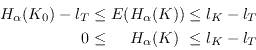
which gives some kind of picture of how the entropies of the final key are distributed. Note that
6.4.1 The problem
If Alice and Bob wish to authenticate a stream of messages and are concerned about Eve's chances to forge any message in the long run the average value doesn't matter much. The average entropy might give an idea of the total chance of forgery, but if she gets infinitely many opportunities for an attack, even if she only can make one active attack, only the minimum possible entropy matters.
As an example, suppose Eve receives information that makes one
of the keys twice as likely as before, while all other keys still
have the same probability as each other. That is, the initial key
![]() is the random
variable
is the random
variable
![]() .
Since the highest probability has doubled, the min-entropy of the
key is reduced by exactly 1 bit. When she sees a message/tag pair
she will rule out all but the
.
Since the highest probability has doubled, the min-entropy of the
key is reduced by exactly 1 bit. When she sees a message/tag pair
she will rule out all but the
![]() keys consistent with the pair. If the more probable key is not
among those, the entropy of the resulting key
keys consistent with the pair. If the more probable key is not
among those, the entropy of the resulting key ![]() will be maximal,
will be maximal, ![]() , since she has no
information about those keys. If the more probable key is among
those left, the new maximal probability is given by renormalizing
the probability
, since she has no
information about those keys. If the more probable key is among
those left, the new maximal probability is given by renormalizing
the probability
![]() .
.
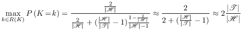 |
(6.5) |
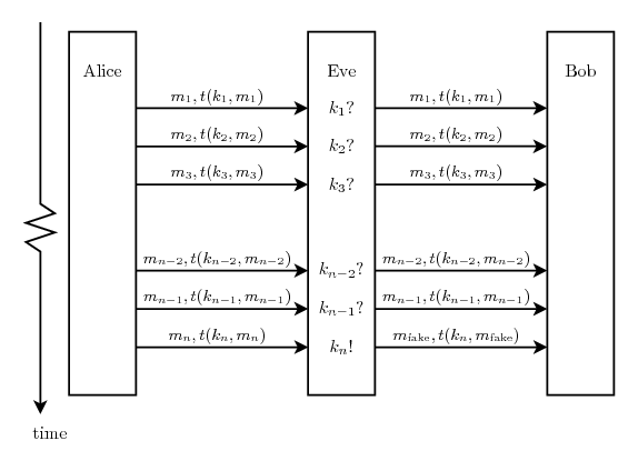
The probability of the most likely key is still approximately twice as high as if Eve had no information at all, which like before means her min-entropy is reduced by 1 bit. Thus, in this case 1 bit of reduced min-entropy in the initial key gives Eve normally no information about the final key and sometimes approximately 1 bit of reduced min-entropy of the final key. The message in the message-tag pair does not matter in this case. Eve's maximum active chance of forgery is just doubled.
As another example, suppose Eve's knowledge of the initial key
![]() is that out of
the
is that out of
the
![]() possible keys, she has a
list of
possible keys, she has a
list of
![]() keys that she knows are not the real one. Furthermore, all those
keys select hash functions that take Alice's message to the same
tag.
keys that she knows are not the real one. Furthermore, all those
keys select hash functions that take Alice's message to the same
tag.
The entropy for this key is very close to the entropy of a
completely unknown key, which is the same thing as the length of
the key. Since the distribution is uniform the Rényi entropy
does not depend on ![]() so we have for any
so we have for any ![]()
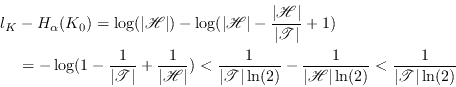 |
(6.6) |
which is pretty small. A realistic tag size might be 32 bits, which would mean that the entropy is reduced with less than four billionths of a bit. Nevertheless, if the tag Alice sends is the right one, Eve will know the key with total certainty and
Eve's active chance of forgery is exactly 1 in this case. If
the message is changed to one where the
![]() keys with 0 probability instead are spread out as evenly as
possible over the
keys with 0 probability instead are spread out as evenly as
possible over the
![]() tags, Eve's entropy for the
final key is independent of both the tag and
tags, Eve's entropy for the
final key is independent of both the tag and ![]() and is bounded by
and is bounded by
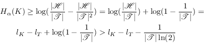 |
(6.7) |
which leaves her maximum active chance of forgery pretty much unaffected when Alice sends this particular message.
6.4.2 The solution
We have seen that simply sending a tag along with each message to prove authenticity does not work in the long run if Eve has a small but non-zero knowledge of the authentication key used. However, only minor adjustments are needed to make Eve's active chance of forgery equal to her passive chance, and therefore makes her chances of successful forgery before being detected equal to her maximum total chance of forgery.
One theoretical solution is for Alice and Bob to have synchronized clocks and agree before each message at which time the message should arrive. At that time Alice will send the message, wait for a time interval longer than the precisions of their clocks, and send the tag. Eve will not know if she will be able to forge a message/tag pair before she sees the real tag, but by then it will be too late to change the message. Keeping the clocks synchronized and agreeing upon fixed times for messages seem kind of problematic though, so this is probably not a good idea.
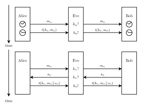
|
A simpler solution that does not need clocks is for Alice to send the message to Bob, who replies with a random fix-sized temporary bit string, called the salt, which Eve must not be able to guess before she sees it. Alice calculates a tag based on the concatenation of the message and the salt and sends that tag to Bob. Before Eve has seen the tag she will not know if she will be able to forge a message/salt/tag triplet, and she will not see the tag before she sends the salt to Alice. Since she cannot send fake salt to Alice and be sure to get away with it before she has seen the real tag, she can either send the real message to Bob and fail but stay undetected or send Alice faked salt and Bob a faked message and with only a very small probability be able to send Bob the right tag. With almost certainty the tag she receives from Alice won't give her enough information so she will probably get caught. This solution requires slightly more time for Alice and Bob to communicate and, since the message to be authenticated now includes the salt, a slightly larger authentication key.
7. Authentication in QKG
As we saw in Section 2.6, a QKG system with a limited lifetime can only generate a limited amount of shared secret key and can be replaced with a pregenerated courier delivered shared key with increased security. Some of the messages of each round need to be authenticated and once the initial key is used a key generated in previous rounds needs to be used. Section 1.2 explains why Eve will have a small but non-zero amount of information about that key.
In Chapter 6 the method of encrypting the authentication tags proposed by Wegman and Carter is shown to be unsuitable when completely secret keys are not available. Using that method in a QKG system would each round give Eve more knowledge about the hash function, which would limit the lifetime of the system to the time when she is expected to know enough to launch an attack.
Chapter 4 gave many examples of the dangers of good security only on average. Chapter 6 reveals that even if Eve initially has very little information about the authentication key, when she has seen Alice's message/tag pair only the expectation value of her knowledge is bounded. If we assume that the authentication tag is sent along with the message and that Eve only needs to forge one message to gain enough power over the key growing process to be able to forge the next message, the risk that Eve is in control of the QKG system will increase for each round and approach unity without Eve ever risking being detected. This would put a theoretical limit to the lifetime of the system.
Fortunately simple solutions exist and two of them are also presented in Chapter 6. They both force Eve to make her attack before she knows that it will succeed by making sure Alice will not send the authentication tag until either Bob has received the message or Eve has done something that would reveal her if she cannot produce the correct tag for her forged message. A QKG system might already have similar properties since a round normally consists of a dialogue of several messages and an authentication tag for all of them at the very end of the round. Whether that is enough to keep the system secure depends on the details of the system, but implementing one of the solutions is cheap and requires no deep analysis of the system.
Finally note that the proposed solutions only makes the authentication secure if Eve's initial knowledge of the key is limited. If the privacy amplification only limits her average knowledge of the authentication key, she will eventually know enough of the key to safely launch an attack regardless of the details of the authentication process.
A. Source code
Bibliography
- 1
- Chip Elliott.
Building the quantum network.
New J. Phys., 4:46, 2002. - 2
- Nicolas Gisin, Grégorie Ribordy, Wolfgang Tittel, and
Hugo Zbinden.
Quantum cryptography.
Rev. Mod. Phys., 74:145-195, 2002. - 3
- Norbert Lütkenhaus.
Estimates for practical quantum cryptography.
Phys. Rev., A59:3301-3319, 1999. - 4
- C. H. Bennett and G. Brassard.
Quantum cryptography: Public key distribution and coin tossing.
In Proc. of the IEEE Int. Conf. on Computers, Systems, and Signal Processing, Bangalore, India, pages 175-179, New York, 1984. IEEE. - 5
- Andrew S. Tanenbaum.
Computer Networks.
Prentice-Hall, third edition, 1996. - 6
- Christian Cachin.
Entropy Measures and Unconditional Security in Cryptography.
PhD thesis, Swiss Federal Institute of Technology Zürich, 1997. - 7
- C. E. Shannon.
A mathematical theory of communication.
Bell Sys. Tech. J., 27:379-423, 623-656, 1948. - 8
- J.L. Massey.
Guessing and Entropy.
In IEEE International Symposium on Information Theory, page 204, Trondheim, Norway, 1994. - 9
- C. H. Bennett, G. Brassard, C. Crepeau, and
U. M. Maurer.
Generalized privacy amplification.
IEEE Transactions on Information Theory, 41(6, Part 2):1915-1923, November 1995. - 10
- Oxford University Press, editor.
The Concise Oxford English Dictionary.
Oxford University Press, eleventh edition edition, 2004. - 11
- Bruce Schneier.
Applied Cryptography.
John Wiley & Sons, Inc., New York, NY, USA, 1993. - 12
- M. N. Wegman and J. L. Carter.
Universal classes of hash functions.
Journal of Computer and System Sciences, 18:143-154, 1979. - 13
- M. N. Wegman and J. L. Carter.
New hash functions and their use in authentication and set equality.
Journal of Computer and System Sciences, 22:265-279, 1981. - 14
- N. Ferguson and B. Schneier.
Practical Cryptography.
Wiley Publishing, Inc., 2003. - 15
- D. R. Stinson.
Universal hashing and authentication codes.
In Joan Feigenbaum, editor, Advances in Cryptology - Crypto '91, pages 74-85, Berlin, 1991. Springer-Verlag.
Lecture Notes in Computer Science Volume 576.
Footnotes
- ... attack2.1
- Not to be confused with what is usually called a Trojan horse attack in computer security.
- ... concave3.1
- Sometimes convex is called
convex-
 and concave is called convex-
 .
. - ... bits4.1
- Note that if the only channel available can only transmit bits, the value must be rounded up to the nearest whole bit.
- ... l'Hospital's4.2
- L'Hospital is nowadays often spelled l'Hôpital.
- ... cards4.3
- This was published in 1948. Information storage has evolved quite a bit since.
- ...tag5.1
- Often called Message Authentication Code, MAC.
- ... Bob5.2
- In the case of digital signatures, Bob can validate the tag but he can not compute it before he has seen it. With symmetrical message authentication Bob can both calculate and validate the tag.
- ....5.3
- Many other functions than XOR will also work, but XOR is normally used in examples.
- ... families5.4
- They are sometimes called classes or sets instead of families.
- ... degree5.5
- Polynomials of higher degree are also possible and usable.
When allowing all polynomials of degree less than
 a strongly
universal
a strongly
universal family is created.